
SEJTA 0.0: Vectors, Matrices, and Tensors - Oh My!
From Foundations to Frontiers: A Software Engineer’s Journey Through AI
Welcome to the inaugural post of our Mathematical Foundations series for A Software Engineer’s Journey Through AI or SEJTA for short (pronounced SAY-TAH). Today, we’re going to be talking about linear algebra—the language that underpins most machine learning algorithms. No matter what area of AI/ML you’re working in, a solid grasp of vectors, matrices, and tensors is indispensable. In this post, we’ll cover the basics of these data structures and give you some resources if you’d like to dig deeper. Practical implementations will be using NumPy and PyTorch.
If you’d like to follow along with the code samples in this post, you’ll need to install some python libraries:
$ pip install torch numpy matplotlib
But First…
Before we get into today’s post, I want to talk to you about NordVPN.
In today’s digital age, safeguarding your online privacy is essential. NordVPN is one of the fastest VPNs in the world and ensure your data remains protected from prying eyes. With over 7,400 servers in 118 countries, fast connection speeds, and a strict no-logs policy, NordVPN is a trusted choice for internet users worldwide. I’ve personally been using NordVPN since 2017 and I can’t recommend it enough!
Click here to visit NordVPN today and help support us!

A Note on Performance
If you’re anything like me, you may be appalled to learn that the majority of AI/ML code is written in python. When I first heard this, I remember wondering how on Earth python would be fast enough for that. I later learned that python modules don’t have to be written in python. In fact, the code that needs the most performance is typically written in C/C++ with python bindings, which is why it’s still so fast despite being used in an interpreted language.
Another important note: these libraries are often about as fast as possible. In many cases, immense amounts of optimization work has been put in to make them even faster. I say this for two reasons:
- To put your mind at ease
- To urge you to use a library rather than implement an algorithm yourself
That’s not to say implementing an algorithm is foolish, quite the contrary, it’s a great learning exercise. But if you’re looking for performance, a widely used library like PyTorch or NumPy is usually going to be about as fast as you’re going to get. If you need even more performance, PyTorch has a C++ binding as well.
Why Linear Algebra Matters in AI
At its core, artificial intelligence is about transforming data. Linear algebra provides the framework for these transformations by enabling us to represent data as mathematical constructs, which can then be manipulated using well-defined mathematical operations. Consider the image recognition algorithms in self-driving cars or the recommendation systems at Netflix, Hulu, YouTube, etc.; from a high-level, these are just fancy applications of linear algebra.
In this post, we’ll explore:
- Vectors: The fundamental building blocks of data representation.
- Vector Spaces: The mathematical foundation that defines what a vector is and what you can do with them.
- Matrices: Tools for organizing and transforming multi-dimensional data.
- Tensors: Generalization of vectors and matrices to higher dimensions.
By the end of this post, you should have a workable understanding of what they are and how to use and manipulate them in Python.
What is Linear Algebra?
Linear algebra is the branch of mathematics concerning vector spaces and linear mappings between these spaces. It provides the language and framework to describe and solve systems of linear equations, which are ubiquitous in AI. It also forms the backbone of many algorithms from things like dimensionality reduction to solving for parameters in a regression model.
- Vector Spaces: Collections of vectors where vector addition and scalar multiplication are defined.
- Linear Transformations: Functions that map vectors to other vectors while preserving vector addition and scalar multiplication.
- Matrices: Compact representations of linear transformations, often used to store data and perform computations efficiently.
Many breakthrough machine learning methods, including deep learning, are built upon layers of linear transformations followed by non-linear activations. In essence, every neural network is a layered tapestry of linear algebra.
Vectors: Building Blocks of Data Representation
In linear algebra, a vector is an ordered list of numbers. It can represent a point in space, a direction, or abstract quantities such as the features of a dataset. The beauty of vectors lies in the mathematical operations you can perform on them. Just to name a few important ones: 1. Addition: Combine two vectors by adding their corresponding components.
- Scalar Multiplication: Multiply each component of a vector by a scalar.
- Dot Product: Measure the similarity between two vectors, which is key in calculating angles and projections.
- Norm: The length or magnitude of a vector. There are many different norms, but the euclidean or L2 norm is the most common.
Now, let’s see a few vector operations in action using Python and NumPy.
import numpy as np

# Define two vectors
v1 = np.array([1, 2, 3])
v2 = np.array([4, 5, 6])

# Compute some operations
v_sum = v1 + v2
v_scaled = 5 * v1
v_dot = np.dot(v1, v2)
v_norm = np.linalg.norm(v1)

print("Vector Sum:", v_sum)
print("Scaled Vector:", v_scaled)
print("Vector Dot Product:", v_dot)
print("Vector Norm:", v_norm)
If you run the above code, you should get an output like this:
Vector Sum: [5 7 9]
Scaled Vector: [ 5 10 15]
Vector Dot Product: 32
Vector Norm: 3.7416573867739413
Vector Spaces: The Foundation Underlying Vectors
So far we’ve only seen vectors as simple lists of numbers, but it’s important to recognize that they reside in a much richer mathematical structure called a vector space. A vector space provides the context in which vectors operate, defining the rules for how we can add them together and scale them with numbers.
A vector space V over a field 𝔽 (commonly the real numbers ℝ in AI applications) is a set of vectors that satisfies the following axioms for every pair of vectors u, v ∈ V and every scalar a, b ∈ 𝔽:
-
Closure under Addition: u + v ∈ V.
-
Commutativity of Addition: u + v = v + u.
-
Associativity of Addition: (u + v) + w = u + (v + w).
-
Existence of an Additive Identity: There exists a zero vector 0 such that u + 0 = u.
-
Existence of an Additive Inverse: For every u ∈ V, there exists a vector -u such that u + (-u) = 0.
-
Closure under Scalar Multiplication: au ∈ V.
-
Compatibility of Scalar Multiplication: a(bu) = (ab)u.
-
Identity Element of Scalar Multiplication: 1u = u (where 1 is the multiplicative identity in 𝔽).
-
Distributivity over Vector Addition: a(u + v) = au + av.
-
Distributivity over Field Addition: (a + b)u = au + bu.
These properties ensure that the structure of the vector space is predictable and robust—allowing us to perform linear combinations and analyze transformations systematically.
In AI/ML, the one you’ll see most often is: ℝn: The set of all n-tuples of real numbers (e.g., ℝ2 or ℝ3) is a vector space. This is the most common setting in machine learning, where data points are represented as vectors.
Think of vector spaces like a stage where performers (vectors) can move in specific directions. Any combination of these moves (vector addition and scalar multiplication) keeps performers on stage. A basis is like choreographed moves that enable reaching any spot on stage. A subspace is a designated region on stage where movements remain confined.
Let’s look at a practical example. While high-dimensional spaces can be abstract, we can easily visualize operations in ℝ2:
import numpy as np
import matplotlib.pyplot as plt

# Define two vectors in R^2
v1 = np.array([2, 3])
v2 = np.array([4, 1])

# Perform scalar multiplication
scalar = 2
v1_scaled = scalar * v1

# Perform vector addition
v_sum = v1 + v2

# Plotting the vectors
origin = [0, 0]  # origin point
plt.quiver(*origin, *v1, color='r', angles='xy', scale_units='xy', scale=1, label='v1')
plt.quiver(*origin, *v2, color='g', angles='xy', scale_units='xy', scale=1, label='v2')
plt.quiver(*origin, *v1_scaled, color='b', angles='xy', scale_units='xy', scale=1, label='2*v1')
plt.quiver(*origin, *v_sum, color='purple', angles='xy', scale_units='xy', scale=1, label='v1+v2')
plt.quiver(*v1, *v2, color='g', angles='xy', scale_units='xy', scale=1, label='v2 moved')
plt.quiver(*v2, *v1, color='r', angles='xy', scale_units='xy', scale=1, label='v1 moved')

plt.xlim(-1, 8)
plt.ylim(-1, 8)
plt.xlabel('X-axis')
plt.ylabel('Y-axis')
plt.title('Vector Operations in R^2')
plt.legend()
plt.grid(True)
plt.show()
When you run this code, you should see something like this:
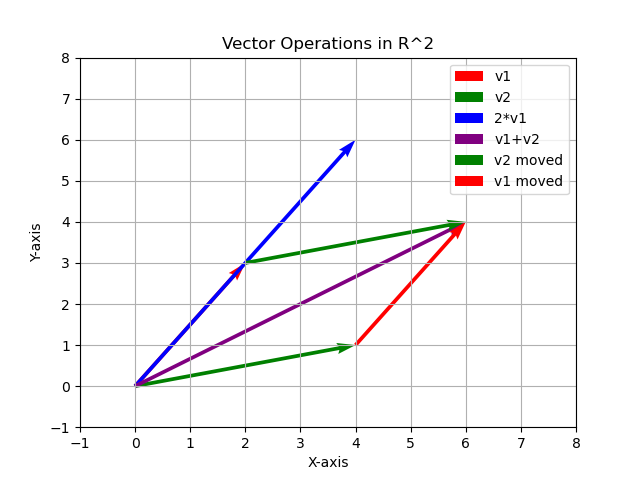
Notice that v1 + v2 is the result of combining v1 and v2 in tip-to-tail fashion and that it doesn’t matter which order this is in (property #2 of vector spaces).
Every vector, matrix, and tensor (we’ll talk about those last two next) operates within the confines of a vector space, ensuring consistency and predictability in our computations.
Matrices: Representing Data and Transformations
Understanding Matrices
Matrices are essentially collections of vectors organized into rows and columns. They serve as efficient data structures for representing datasets and performing linear transformations. In AI, matrices are ubiquitous. They’re used for everything from storing pixel values of images to representing weights in neural networks.
Basic Matrix Operations
- Matrix Addition: Element-wise addition of two matrices, both matrices must be the same size.
- Matrix Multiplication: Combines rows and columns to produce a new matrix. Matrices must have compatible sizes (an
m×nmatrix can be multiplied by ann×pmatrix resulting in anm×pmatrix). Note that multiplication is not commutative, soAB ≠ BA. - Transpose: Flips a matrix over its diagonal.
- Inverse: A matrix that, when multiplied with the original, yields the identity matrix (if it exists).
Let’s illustrate matrix multiplication and other operations using NumPy:
# Define two matrices
A = np.array([[1, 2], [3, 4]])
B = np.array([[5, 6], [7, 8]])
print("Matrix A:\n", A)
print("Matrix B:\n", B)

# Matrix multiplication
C = np.dot(A, B)
print("Matrix Product:\n", C)

# Matrix addition
D = A + B
print("Matrix Sum:\n", D)

# Transpose of a matrix
A_transpose = np.transpose(A)
print("Transpose of A:\n", A_transpose)

# Inverse of a matrix (if it exists)
A_inverse = np.linalg.inv(A)
print("Inverse of A:\n", A_inverse)
If you run the above code, you should get something like this:
Matrix A:
 [[1 2]
 [3 4]]
Matrix B:
 [[5 6]
 [7 8]]
Matrix Product:
 [[19 22]
 [43 50]]
Matrix Sum:
 [[ 6  8]
 [10 12]]
Transpose of A:
 [[1 3]
 [2 4]]
Inverse of A:
 [[-2.   1. ]
 [ 1.5 -0.5]]
Tensors: Extending the Concepts of Vectors and Matrices
Vectors and matrices serve as powerful tools, but many real-world AI applications involve data with even more dimensions. This is where tensors come into play—extending the concept of scalars (0-dimensional), vectors (1-dimensional), and matrices (2-dimensional) to handle higher-dimensional data.
What Exactly Is a Tensor?
Simply put, a tensor is a multi-dimensional array that generalizes scalars, vectors, and matrices:
- A scalar (e.g., temperature reading) is a 0-dimensional tensor.
- A vector (e.g., feature vector of an object) is a 1-dimensional tensor.
- A matrix (e.g., grayscale image data) is a 2-dimensional tensor.
- Higher-dimensional tensors (3D or greater) can represent more complex structures:
- A 3-dimensional tensor can represent an RGB image, where dimensions correspond to height, width, and color channels.
- A 4-dimensional tensor might represent video data (frames, height, width, color channels).
Tensors provide a unified abstraction, simplifying operations and enabling efficient computations on modern hardware (e.g., GPUs).
Basic Tensor Operations
Common tensor operations you’ll encounter include:
- Element-wise Operations: Apply mathematical operations independently to each element.
- Reshaping: Changing tensor dimensions without altering data, reorganizing how it’s viewed or accessed.
- Slicing and Indexing: Extract specific portions of a tensor.
- Reduction Operations: Summarizing a tensor along one or more dimensions (e.g., summation, averaging).
Here’s how you can perform some of these operations with PyTorch:
import torch

# Creating tensors
tensor_3d = torch.tensor([[[1, 2], [3, 4]],
                          [[5, 6], [7, 8]]])

# Element-wise multiplication
tensor_squared = tensor_3d ** 2

# Reshaping a tensor
tensor_reshaped = tensor_3d.view(2, 4)

# Slicing a tensor
tensor_slice = tensor_3d[:, 0, :]

# Reducing tensor dimensions (e.g., summation)
tensor_sum = torch.sum(tensor_3d, dim=0)

print("Original 3D Tensor:\n", tensor_3d)
print("Squared Tensor:\n", tensor_squared)
print("Reshaped Tensor (2x4):\n", tensor_reshaped)
print("Sliced Tensor:\n", tensor_slice)
print("Summation along dimension 0:\n", tensor_sum)
Running this code will give you something like this:
Original 3D Tensor:
 tensor([[[1, 2],
         [3, 4]],

        [[5, 6],
         [7, 8]]])
Squared Tensor:
 tensor([[[ 1,  4],
         [ 9, 16]],

        [[25, 36],
         [49, 64]]])
Reshaped Tensor (2x4):
 tensor([[1, 2, 3, 4],
        [5, 6, 7, 8]])
Sliced Tensor:
 tensor([[1, 2],
        [5, 6]])
Summation along dimension 0:
 tensor([[ 6,  8],
        [10, 12]])
Why Are Tensors Important in AI?
Tensors are foundational to modern neural networks. They enable efficient computation, which is vital when dealing with massive datasets or complex models. Here are a few specific examples:
- Convolutional Neural Networks (CNNs):
- CNNs use tensors to represent images and convolutional kernels. A typical input tensor for CNNs has dimensions corresponding to (batch_size, channels, height, width). Convolution operations and pooling layers manipulate these tensors to extract meaningful features.
- Natural Language Processing (NLP):
- NLP tasks utilize tensors to represent sequences of words or tokens as vectors. For example, transformer models process data as tensors with dimensions corresponding to (batch_size, sequence_length, embedding_dimension).
- Recommendation Systems:
- Recommendation algorithms can model user-item interactions as higher-dimensional tensors, capturing user preferences across contexts like time, location, or device type.
Let’s look briefly at how tensors appear in practical scenarios:
- Color Images:
A 256x256 RGB image can be represented as a tensor with shape(3, 256, 256), where each channel holds pixel intensity values. - Videos:
Video data can be represented as a tensor with dimensions(frames, channels, height, width), capturing spatial and temporal information. - Medical Imaging (MRI or CT scans):
Often stored as 3D or even 4D tensors, these medical images represent multiple layers of spatial data, and potentially temporal sequences of scans.
Tensors are the backbone of modern AI computations, offering a unified abstraction, computational efficiency, and versatility. As we delve deeper into advanced AI/ML concepts in upcoming posts, you’ll see tensors repeatedly emerge as the core structure behind many algorithms.
Practical Applications
So you understand vectors, matrices, and tensors now, but what does it all mean practically? Let’s look at a few real-world use-cases for these constructs:
- Image Processing: Remember how we mentioned representing images as tensors? Each pixel’s color value (Red, Green, Blue) can be represented as a number in a tensor, with an 8-bit integer (0-255) for each component being the most common. Operations like blurring, sharpening, and edge detection are all computed using matrix operations.
- Natural Language Processing (NLP): Words can be embedded as vectors using techniques like Word2Vec (we’ll talk about these techniques in a future post). This allows AI models to understand semantic relationships. The similarity between these word vectors can tell you how similar two pieces of text are.
- Robotics: Rotations and translations can be used to control a robot’s movements - and these operations, linear transformations, can be represented using matrices.
- Dimensionality Reduction: Sometimes, datasets have too many features and models have a hard time learning from the information overload. Techniques like Principal Component Analysis (PCA) use eigenvalues and eigenvectors to reduce the number of dimensions while retaining the most important information.
The key takeaway here is that linear algebra provides a common language for describing and manipulating data across a wide range of applications. Once you understand the underlying math, you can start to see the connections between seemingly disparate fields.
Tips and Takeaways
Alright, time for some practical advice to solidify your understanding. The best way to do that is to think critically about the material, ask questions, and practice.
- Start with Visualization: Linear algebra can feel abstract. Use tools like matplotlib (as shown in the examples) to visualize vectors. Plotting things out can make the concepts much more intuitive.
- Play with NumPy and PyTorch: The best way to learn is by doing. Experiment with different vector and matrix operations in Python. Try to recreate some of the examples from this post, and then try to modify them.
- Don’t Reinvent the Wheel (Initially): As mentioned earlier, use optimized libraries like NumPy and PyTorch for your computations. Focus on understanding how to use them first and building an intuition about what it’s doing. Later, if you’re feeling ambitious, you can dive into the implementation details.
- Ask Questions: Understanding linear algebra is not just about memorizing formulas. It’s about building an intuition for how data is transformed. As yourself:
- How does a change in a matrix cell value impact the result of multiplying it with another matrix?
- Scalars and matrices have inverses, what about vectors and tensors?
Revisit these concepts regularly. As we progress to more advanced topics like neural networks, deep learning, or reinforcement learning, you’ll find that a firm grasp of linear algebra serves as an invaluable tool in your toolkit.
A Foundation for the Future
In this post, we journeyed through the essential components of linear algebra—from the basics of vectors and matrices to the generalization with tensors. These concepts are going to be very important in understanding data and data manipulation techniques used in AI/ML.
As we move forward in this series, we’ll continue building on the mathematical framework needed to understand classical machine learning techniques, neural network architectures, and many others. For those interested in digging deeper, consider checking out the related links at the bottom of this post.
Remember: a strong mathematical foundation is the secret sauce that turns theory into breakthrough applications. Until next time, keep exploring, coding, and innovating.
Related Links:
- Linear Algebra: Foundations to Frontiers (LAFF)
- Linear Algebra: Khan Academy
- NumPy Linear Algebra documentation
- 3Blue1Brown: Essence of Linear Algebra (YouTube) (Excellent visual explanations)
Keywords: Linear Algebra, AI, Vectors, Matrices, Eigenvalues, Eigenvectors, SVD, Machine Learning, Python, NumPy