
SEJTA 0.1: May the Stats Be With You
From Foundations to Frontiers: A Software Engineer’s Journey Through AI
Welcome to the second post of our Mathematical Foundations series for A Software Engineer’s Journey Through AI (SEJTA for short, pronounced SAY-TAH). Today, we’ll be talking about probability and statistics, the language of uncertainty. We’ll gain an understanding of how to quantify and manage uncertainty in the chaotic world we live in. Hopefully by the end of this post, you’ll have a solid grasp of the basics of probability theory and estimation.
If you’d like to follow along with the code samples in this post, you’ll need to install some python libraries:
$ pip install torch numpy matplotlib
But First…
Before we get into today’s post, I want to talk to you about NordPass.
Secure your digital life effortlessly with NordPass, the advanced password manager designed to simplify online security without compromising on power. Built on cutting-edge XChaCha20 encryption and a zero-knowledge architecture, NordPass ensures that only you have access to your sensitive data, whether it’s passwords, credit card details, or secure notes. Its intuitive design, seamless autofill, and smart password generator make managing your login credentials a breeze, while premium features like password health assessments, data breach monitoring, and email masking provide an extra layer of protection against cyber threats.
Click here to get NordPass today and help support us!

Why are Probability & Statistics Important?
Wouldn’t it be nice if we could use AI/ML to model our world perfectly? Unfortunately, that’s not the case. The real world and our measurements of it are often filled with uncertainty and noise. Luckily, we don’t always need to model the world perfectly. In many cases, (probably) close is good enough. Most of the time, we still need to know how uncertain our data is or likely our predictions are. For that, we use statistics. Probability theory deals with predicting the likelihood of future events based on known distributions or assumptions. Statistics, in contrast, primarily involves analyzing observed data to infer underlying patterns or characteristics. Probability provides tools used extensively within statistics. By employing probability theory, we can:
- Describe how likely different outcomes are.
- Use data to estimate unknown quantities.
- Determine if observations are statistically significant.
When I took my first Deep Learning class, I had never taken a statistics class despite my math background. The majority of the math classes I had taken up until that point were calculus-based, most of which had no uncertainty in the material. In this post, I hope to give you the information that would have helped me tremendously in my first Deep Learning class.
Probability Theory
As I mentioned above, probability is a subset of statistics that deals with likelihood. Probability theory is the study of, well, probability! Whether you realize it or not, you encounter probabilities all the time:
- Forecasts: Weather forecasts aren’t certain, they’re predictions of what’s most likely to occur based on the information the forecaster had at the time of prediction.
- Traffic Lights: Traffic signals often give statistical priority to certain directions depending on vehicle frequency.
- Shopping Recommendations: If you’ve ever gotten a recommendation for a product from a retailer, their system determined you had a high likelihood of liking that product based on your shopping patterns as compared to others who bought that product.
The probability of an event is simply the chance it will occur. If you flip a coin, there’s a 50% chance it will land on heads and a 50% chance it will land on tails. Mathematically speaking: P(Heads) = 0.5 = P(Tails). This syntax will be important to know later. P(X) = p simply means the probability of event X occurring is p, where p is a real number between 0 and 1. In probability, 0 means an event will never occur (0%) and 1 means an event definitely will (100%).
A probability can also be conditional: P(X | Y) = p. This just means that the probability of X occurring given that Y is true, is p. If you have some other information, you can calculate the conditional probability:

Here, P(A ∩ B) is the probability of both A and B being true. Let’s look at a concrete example of this. Suppose there is some medical test that has a 90% accuracy of testing for a certain disease. Let’s assume this disease is present in 1% of the population. If you test positive for this disease (P(Disease | Positive Test)), what is the probability you actually have it? Plugging in some numbers, we get:

In order to solve this, we need a few things:
P(Disease and Positive)- This is the probability of having the disease and testing positive (true positive). With a 1% incidence rate and 90% accuracy, this is0.01 * 0.9 = 0.009.P(Positive)- This one’s a bit more involved. The probability of testing positive, regardless of whether you have the disease at all, is sum of the probability of testing positive with the disease (true positive) and the probability of testing positive without the disease (false positive). In our example, this is0.01 * 0.9 + 0.99 * 0.1 = 0.108.
Now we can solve P(Disease | Positive):

That means, in our example, a positive test means you only have an 8.3% chance of having the disease - much better than 90%!
Let’s take a wider view now, and talk about distributions. A probability distribution describes how likely different outcomes are when dealing with random events. It gives each possible outcome a chance expressed as a number between zero and one. When you look at all possible outcomes together, their probabilities always add up exactly to one. Probability distributions help you understand which results are common and which ones rarely happen. There are two types of distributions we usually care about: continuous and discrete distributions.
Continuous probability distributions apply when you deal with outcomes measured along a range, where any value within that range is possible. For example, the height of people in a population can be described by a continuous distribution. The response time of an API would also be a continuous distribution. With this type of distribution, it’s relatively easy to compute the probability of falling within a certain interval or range. Some of the more common continuous distributions you’ll encounter in AI/ML:
- Normal Distribution: Very common in real-world data, many algorithms assume data follows a normal distribution.
- Uniform Distribution: Assigns an equal probability to every value in the given range. Often used in random initialization and random number generation.
Discrete probability distributions apply when outcomes are countable and discrete (or separate), like whole numbers. The number of SMS messages people in a group send per day would be an example of this. Each outcome has a clearly defined probability. Some of the more common discrete distributions you’ll encounter in AI/ML:
- Bernoulli Distribution: Represents simple binary outcomes (0 or 1). This distribution is widely used in classification tasks, modeling binary decisions or events, and as the building block for more complex distributions.
- Binomial Distribution: Extends the Bernoulli Distribution by modelling a system over multiple Bernoulli “trials”. Common in tasks like predicting the number of correct classifications out of a total set of predictions.
The expectation of a random variable is what you would typically anticipate happening over many trials. It’s essentially the average outcome you get if you repeat an experiment or a process many times.
The definition of expectation for discrete distributions is:

For continuous distributions, it’s:

You may also like to know the variance of your data. That tells you how spread out data is around the expected value. Its a great way to get some information about the consistency of either your data or your predictions. The variance is computed using the expectation as:

The standard deviation is closely related to variance, it’s simply the square root of variance. It represents how much, on average, data points deviate from the expectation, measured in the same units as the original data. If variance gives you an abstract measure of spread, standard deviation provides a more intuitive measure of uncertainty in the same units as your data, making it easier to interpret practically.
You typically don’t need to calculate these by hand, numpy can do it for us:
import numpy as np

data = np.array([1, 2, 3, 4, 5])
mean = np.mean(data)
variance = np.var(data)
std_dev = np.std(data)

print(f"Mean: {mean}, Variance: {variance}, Standard Deviation: {std_dev}")
Running this code gives:
Mean: 3.0, Variance: 2.0, Standard Deviation: 1.4142135623730951
Consider again, the sample we used in our discussion of conditional probabilities. We showed a way to calculate the probability of having the disease given a positive test. What if we wanted to invert the question and find the probability that we get a positive test given that we have the disease. Obviously we’d want to have a high likelihood of catching the disease if we actually do have it!
Bayes’ Theorem can help us with that:


Recall, P(A) is the probability of having the disease, P(B) is the probability of testing positive for it, and P(A | B) is the probability of actually having the disease given that we tested positive for it. Using that information, let’s calculate the probability of testing positive, if we have the disease (P(B | A)):

So that means if we have the disease, there’s almost a 90% chance we’ll test positive for it. This is a good example of scenarios where probabilities aren’t always intuitive. If this is you, you’re not alone! Our intuition evolved to keep us alive, it didn’t evolve to help us with Bayes’ Theorem. As such, our gut reaction about a situation like this, how you’d feel hearing these test results, often needs to be checked by the math.
Estimation
In the real-world, data is often messy and noisy. Sometimes the thing we’re trying to measure is chaotic (e.g. weather data). Our measurement tools can also be noisy, either because they’re low quality or the technology is inherently noisy (e.g. gyroscopes).
Because of this, we often need to estimate values for data we’re measuring. A simple way to do that is to average over some small period of time. When getting gyroscope data from a sensor that samples (takes a measurement) at 1kHz, we could average the value over the past 100 samples and get a less chaotic measurement at a lower resolution, one every 100 milliseconds.
Unfortunately, that may not be enough. In the case of gyroscopes, the measurement may drift over time. On short timescales, like 100 samples, you won’t notice it. But over time, the values produced by the sensor may begin to drift in a random direction due to the nature of the sensor itself. A brute force solution is to buy more expensive and higher quality sensors, but:
- A: That may not be possible in every situation
- B: A good enough sensor may exceed your budget
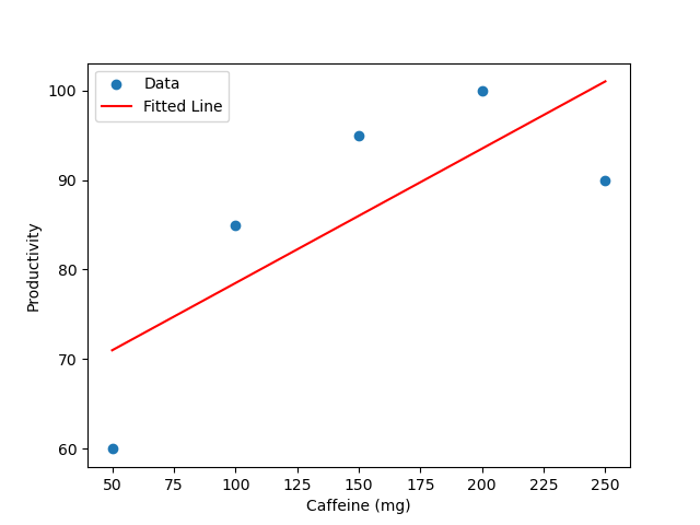
Besides cleaning up noise, you may notice patterns in your data. Let’s say you want to know the optimal caffeine intake for your productivity. If you plot caffeine intake on the X axis and your productivity on the Y axis, you may notice a strong trend line. The Least Squares line is the straight line drawn through the data points so that the vertical distances (errors) from each point to the line are as small as possible. In real life it would probably look like a bell curve instead of a straight line because too much caffeine is more of a hindrance than an enabler but we’ll stick with a line because it’s easier!
Least Squares is an estimation technique we can use to find the best fit for our caffeine-productivity dataset. What we’re doing is linear regression. The goal is to find a line of best fit, one that minimizes the overall difference between our predictions and the actual values. Least squares does this by calculating the squared differences between each prediction and actual data point, then adjusting the parameters to make this total difference as small as possible:

Where

Let’s see what this looks like in code:
import numpy as np
import matplotlib.pyplot as plt

# Sample data (caffeine vs. productivity)
caffeine = np.array([50, 100, 150, 200, 250])
productivity = np.array([60, 85, 95, 100, 90])

# Linear regression using numpy
# Fit a line (degree 1 polynomial)
m, b = np.polyfit(caffeine, productivity, 1)

# Generate points for the fitted line
x_fit = np.linspace(50, 250, 100)
y_fit = m * x_fit + b

print(f"Slope (m): {m}, Intercept (b): {b}")

# Plot the data and the fitted line
plt.scatter(caffeine, productivity, label='Data')
plt.plot(x_fit, y_fit, color='red', label='Fitted Line')
plt.xlabel('Caffeine (mg)')
plt.ylabel('Productivity')
plt.legend()
plt.show()
If you run this code, you should see something like this:
There are other types of regression techniques for data that isn’t linear (e.g. logarithmic, logistic, etc.). For cleaning up noisy data, we use techniques such as Maximum Likelihood Estimation (MLE). In MLE, we assume our data was sampled from a distribution and choose parameters of that distribution that maximize the probability that sampling from it would give us data with the same distribution as our observations.
Bayesian Estimation refers broadly to updating probability estimates as new data is observed. One common Bayesian estimation technique used extensively in robotics and navigation is the Kalman Filter, which combines multiple noisy data sources to increase accuracy.
One last estimation technique I’ll talk about is called Bayesian Estimation. Bayesian Estimation refers broadly to updating probability estimates as new data is observed. One common Bayesian estimation technique used extensively in robotics and navigation is the Kalman Filter, which combines multiple noisy data sources to increase accuracy. Instead of finding a single “best guess” parameter value, you treat it as a probability distribution. We start with an initial “belief” about our data, called a prior, and update this belief over time using our observations.
For example, we could use a GPS module and a gyroscope+accelerometer IMU (Integrated Measurement Unit) attempting to keep track of a robot’s position as it moves throughout the world. Both sensors will have some inaccuracies and stochasticity (randomness) but combining the data of the two using a Kalman Filter provides more accuracy than using either of them individually.
Practical Applications
Understanding probability and statistics is a critical skill for software engineers in the AI/ML field. These mathematical tools enable the modeling and management of uncertainty inherent in real-world data. Here are some practical applications:
- Autonomous Systems: Self-driving cars and robotics use probabilistic models like Kalman Filters to interpret sensor data and make decisions in uncertain environments.
- Recommendation Systems: By analyzing user behavior patterns, probabilistic models predict and suggest products or content that users are likely to prefer.
- Spam Filtering: Email services use probabilistic classifiers to determine the likelihood of a message being spam based on its content and metadata.
Tips and Takeaways
It’s time for some practical advice to solidify your understanding. The best way to do that is to think critically about the material, ask questions, and practice.
- Grasp Fundamental Concepts: Try to get a solid understanding of basic probability and statistics concepts. A good understanding of the basics is 80% of the battle.
- Learn Common Distributions: Familiarize yourself with the commonly used probability distributions we talked about: Normal (Gaussian), Uniform, Bernoulli, and Binomial.
- Apply Bayesian Thinking: Develop an intuition for Bayesian methods to update beliefs based on new data. Not only is this helpful in AI/ML, it’s helpful in every-day life too.
- Practice with Real Data: Engage in projects that involve real-world data to apply probabilistic models and statistical analysis, enhancing practical understanding.
A Foundation for the Future
In this post, we discussed some of the most important concepts in probability and statistics. The tools we talked about will be very useful for understanding uncertainty and dealing with noisy data in AI/ML.
As we move forward in this series, we’ll continue building on the mathematical framework needed to understand classical machine learning techniques, neural network architectures, and many others. For those interested in digging deeper, consider checking out the related links at the bottom of this post.
Remember: a strong mathematical foundation is the secret sauce that turns theory into breakthrough applications. Until next time, keep exploring, coding, and innovating.
Related Links:
- MIT OpenCourseware: Introduction to Probability and Statistics
- StatQuest: Statistics Fundamentals
- 3Blue1Brown: Bayes Theorem
Keywords: Probability, Statistics, Data Science, Machine Learning, AI, Uncertainty, Data Analysis, Inference